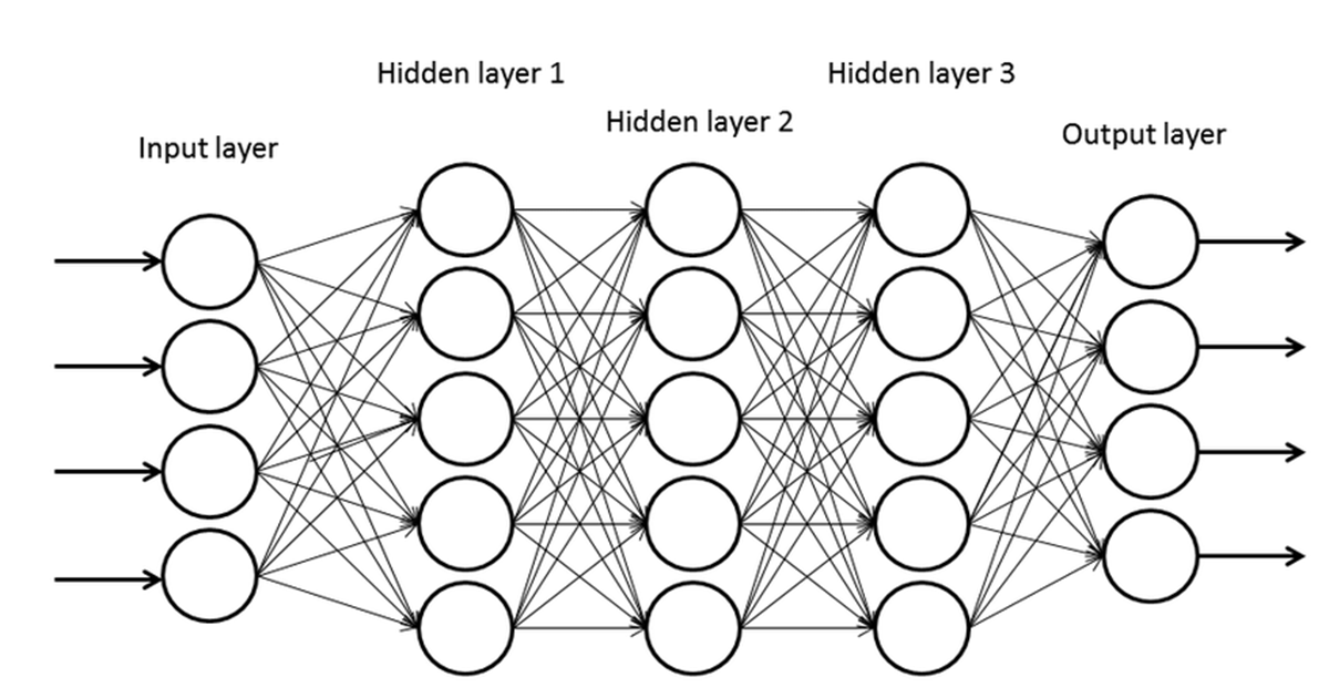
Optimizing Gradient Descent
Contents
Stochastic Gradient Descent
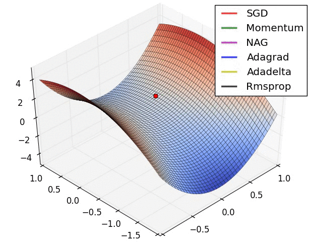
Stochastic gradient descent is a method that accelerates training. For simple models that have few layers and few neurons per cell, vanilla gradient descent (aka batch gradient descent) will run without causing a lot of issues. The problem arises when the scale of the model gets large and complicated. Let’s assume we apply vanilla gradient descent to a neural network that has a layer with 10,000 features. Weight update would look something like this.
$$ w_1 = w_1 - \eta\frac{\partial}{\partial w_1}\sum_{i=1}^n(t_i-y_i)^2 = w_1 - \eta(\frac{\partial E_1}{\partial w_1} + \frac{\partial E_2}{\partial w_1} + … + \frac{\partial E_n}{\partial w_1}) $$ $$w_2 = w_2 - \eta\frac{\partial}{\partial w_2}\sum_{i=1}^n(t_i-y_i)^2 = w_2 - \eta(\frac{\partial E_1}{\partial w_2} + \frac{\partial E_2}{\partial w_2} + … + \frac{\partial E_n}{\partial w_2}) $$ $$ … $$ $$ w_{10000} = w_{10000} - \eta\frac{\partial}{\partial w_{10000}}\sum_{i=1}^n(t_i-y_i)^2 = w_{10000} - \eta(\frac{\partial E_1}{\partial w_{10000}} + \frac{\partial E_2}{\partial w_{10000}} + … + \frac{\partial E_n}{\partial w_{10000}}) $$
Vanilla Gradient Descent
This is the computation for 1 sample. But if we have 10,000 samples, this would mean we would need 100 million calculations just for one epoch, which would take too much time to train.
Stochastic gradient descent addresses this by randomly sampling 1 gradient. Mini batch gradient descent uses a small batch of gradients (usually $2^n$ samples) in each epoch. This statistical approach allows us to estimate the gradient with less computation.
There is some confusion in terminology, but generally, batch gradient descent refers to the standard method that computes gradients over the entire dataset, while stochastic and mini-batch gradient descent refer to methods that compute gradients using a batch size of 1 and n (16, 32, 64, …), respectively.
Since we know that $$ \frac{\partial E}{\partial w_1} = \frac{1}{n}\sum_{i=1}^{n}\frac{\partial E_i}{\partial w_1} $$ we can assume $$ \frac{\partial E}{\partial w_1}\approx\frac{\partial E_1}{\partial w_1}\approx\frac{\partial E_2}{\partial w_1}\approx…\approx\frac{\partial E_n}{\partial w_1} $$ and use this value to substitute the entire sum of gradients.
The pseudocode for stochastic gradient descent is as follows.
Repeat
    for n=1 to N (Entire training dataset)
        w = w - lr * dE_n / dw
    end
This is usually faster than vanilla gradient descent and can also be used for online learning. However, since it uses only 1 sample from the entire set, fluctuations may occur and negatively affect accuracy. Using a small learning rate can be a way to achieve similar performance.
Mini batch gradient descent uses batches of size n (typically numbers that are $2^n$). For 1 epoch, gradients are calculated for each batch.
Repeat
    for b=1 to B (All batches)
        g_sum = 0 # gradient sum
        for n=1 to N (Entire training dataset)
            g_sum += dE_n/dw
        end
        w = w - lr * g_sum
    end
One notable part of the process is that different gradient values are used for each batch. For example, if we set the batch size as 2, the first batch uses $\frac{\partial E_1}{\partial w_m} + \frac{\partial E_2}{\partial w_m}$, the next batch uses $\frac{\partial E_3}{\partial w_m} + \frac{\partial E_4}{\partial w_m}$, and so on. This is because using the same value for every batch will lead to biased results, degrading accuracy.
Stochastic gradient descent and mini batch gradient descent both provide a good estimation of the true gradient and allow high throughput, allowing a large number of GPU cores to be used at once, which enables fast convergence. However, when datasets have high variance, the results may be noisy and inaccurate. Mini batch gradient descent (n samples) usually yields better results and is more stable than stochastic gradient descent (1 sample), but it still differs from batch gradient descent (all samples) in terms of gradient values.
Momentum
The core idea of naive gradient descent is widely used, but they have the drawback that they cannot make progress when the gradient is zero or close to zero. If a point lies near a local minimum, small gradients may not be an issue. However, problems arise when the gradient is close to zero at a point far from any minimum. A common scenario is when a randomly initialized starting point yields very small gradients, stalling optimization.
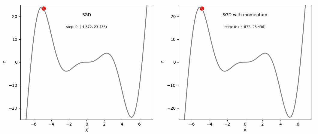
This is where momentum can be applied. Momentum is a technique that improves optimization quality. It can be thought of as a ball that rolls down the loss function. A simple gradient descent method will stop as soon as it reaches a local minimum, but with momentum applied, the point will keep moving even after reaching a local minimum and may reach a lower minimum.
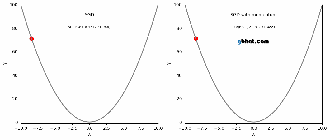
SGD and SGD with Momentum
Momentum is defined by adding a vector in the direction of past weight updates, combining the previous update with the current gradient. $$ m^t = \beta m^{t-1} - \eta g^t $$ $$ w^t = w^{t-1} + m^t $$
- $g^t$: gradient at iteration t
- $\beta$: momentum rate
- $\eta$: learning rate
Momentum can be written as follows. $$ m^t = -\eta(g^t +\beta g^{t-1} + \beta^2g^{t-2} + … + \beta^{t-1}g^1) $$ This is equivalent to saying momentum is the exponential average of past gradients. With momentum, the learning process becomes more stable and consistent.
One advantage of momentum is that it helps escape local minima (although not guaranteed). If we assume a scenario where $g^t$ is a value close to 0, $$ m^t = -\eta(g^t + \beta g^{t-1} + \beta^2g^{t-2} + … + \beta^{t-1}g^1) $$ $$ = -\eta(\beta g^{t-1} + \beta^2g^{t-2} + … + \beta^{t-1}g^1) $$ We can see that even though $g^t$ is 0, the past values have been accumulated and are not 0, meaning it will still update and converge to some local minimum.
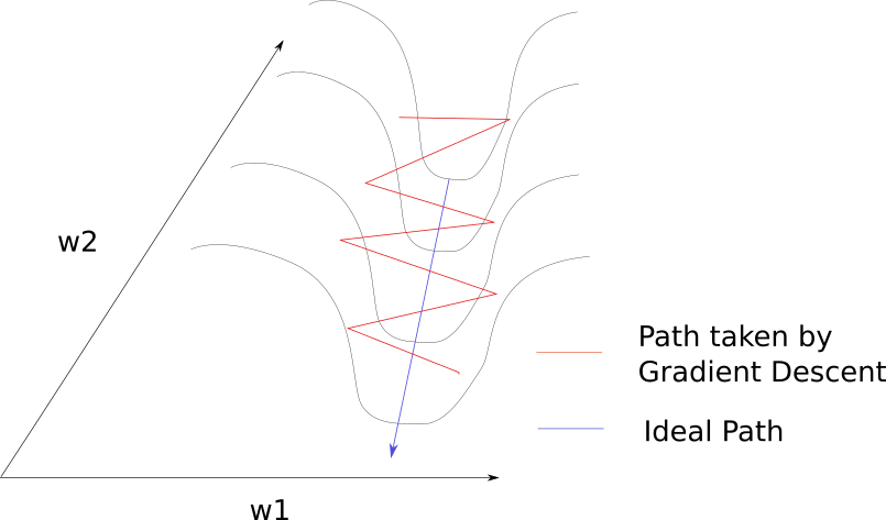
Another advantage is that it allows faster convergence. As mentioned above, gradients are accumulated exponentially, which results in:
- Momentum being amplified in areas where gradient directions are consistent, e.g. shallow directions where gradient values are close to 0.
- A larger learning rate along consistent directions due to exponential accumulation of past gradients.
- Reduced oscillation in steep directions because gradients with alternating signs cancel each other out.
SGD and SGD with Momentum
Adaptive Learning Rates
The learning rate is usually set when designing a model. However, hardcoding this would result in the same constant value for all variables, regardless of each gradient value. This can cause uneven updates, resulting in slow convergence or oscillation.
Assume that we have two features, each with weights $w_1$ and $w_2$. Each weight would be updated as follows. $$ w_1 = w_1 - \eta \frac{\partial E}{\partial w_1} $$ $$ w_2 = w_2 - \eta \frac{\partial E}{\partial w_2} $$ If $w_1$ is updated with big steps and $w_2$ with small steps for a given learning rate, its convergence would be inefficient and may be prone to oscillation, since the learning rate is fixed regardless of the variable and gradient. We can think of it as the point moving along a path that does not directly lead to a local minimum.
Adagrad
One workaround is Adagrad. Adagrad sets different learning rates for different variables by taking into account past gradient values. $$ w^t_i = w^{t-1}_i-\eta g^t_i $$
Standard Gradient Descent
$$ G^t_i=G^{t-1}_i+(g^t_i)^2 $$ $$ w^t_i = w^{t-1}_i-\frac{\eta}{\sqrt{G^t_i+\epsilon}}g^t_i $$
Adagrad
- $g^t_i$: gradient of parameter $i$ at time $t$
- $G^t_i$: accumulated change of parameter $i$ from beginning($\Delta w^t_i$), also accumulated gradients of parameter $i$ from beginning
- $\epsilon$ is added to $G^t_i$ in cases where $G^t_i$ is 0.
Adagrad decreases the learning rate for parameters with large gradients and increases it for those with small gradients. However, since $G^t_i$ increases monotonically, $\frac{\eta}{\sqrt{G^t_i+\epsilon}}$ will eventually reach 0 and weights will not be updated at a certain point.
RMSProp
RMSProp addresses this issue and considers recent updates only. $G^t_i$ is redefined as follows. $$ G^t_i=\gamma G^{t-1}_i + (1-\gamma)(g^t_i)^2 $$ $$ G^t_i = (1-\gamma)[(g^t_i)^2+\gamma(g^{t-1}_i)^2 + \gamma^2(g^{t-2}_i)^2 + … + \gamma^{t-2}(g^2_i)^2 + \gamma^{t-1}(g^1_i)^2] $$ where $0<\gamma<1$. In the second equation, $\gamma^{t-1}, \gamma^{t-2}$ … at some point will become 0, due to accumulated multiplication of a value in range $(0,1)$. Therefore, $\frac{\eta}{\sqrt{G^t_i+\epsilon}}$ will sometimes increase and sometimes decrease depending on recent updates.
Adam
Adam combines RMSProp with momentum and is one of the most frequently used optimizers today. The base definition is as follows. $$ m^t_i = \beta_1m^{t-1}_i - (1-\beta_1)g^t_i $$ $$ G^t_i = \beta_2G^{t-1}_i + (1-\beta_2)(g^t_i)^2 $$ $$ w^t_i = w^{t-1}_i + \frac{\eta}{\sqrt{G^t_i + \epsilon}}m^t_i $$ In practice, $m^t_i$ and $G^t_i$ are replaced with $\hat{m^t_i}$ and $\hat{G^t_i}$ for unbiased expectation. $$ \hat{m^t_i} = \frac{m^t_i}{1-(\beta_1)^t} $$ $$ \hat{G^t_i} = \frac{G^t_i}{1-(\beta_2)^t} $$ $$ w^t_i = w^{t-1}_i + \frac{\eta}{\sqrt{\hat{G^t_i} + \epsilon}}\hat{m^t_i} $$ Finally, below is a famous image of how each optimization method behaves when starting from a saddle point.
Gradient Descent Methods on a Saddle Point
References
Gradient Descent Nesterov Momentum
Intro to optimization in deep learning: Momentum, RMSProp and Adam