Introduction
Perceptrons
Neural Networks
References

Introduction

A neural network is a machine learning model that stacks perceptrons in layers and its structure is inspired by the human brain. The human brain has countless neurons connected into a network, each sending signals to other neurons. While a neural network also aims to follow this structure, it consists of layers with several perceptrons in each layer. This structural choice is due to simplicity in implementation.

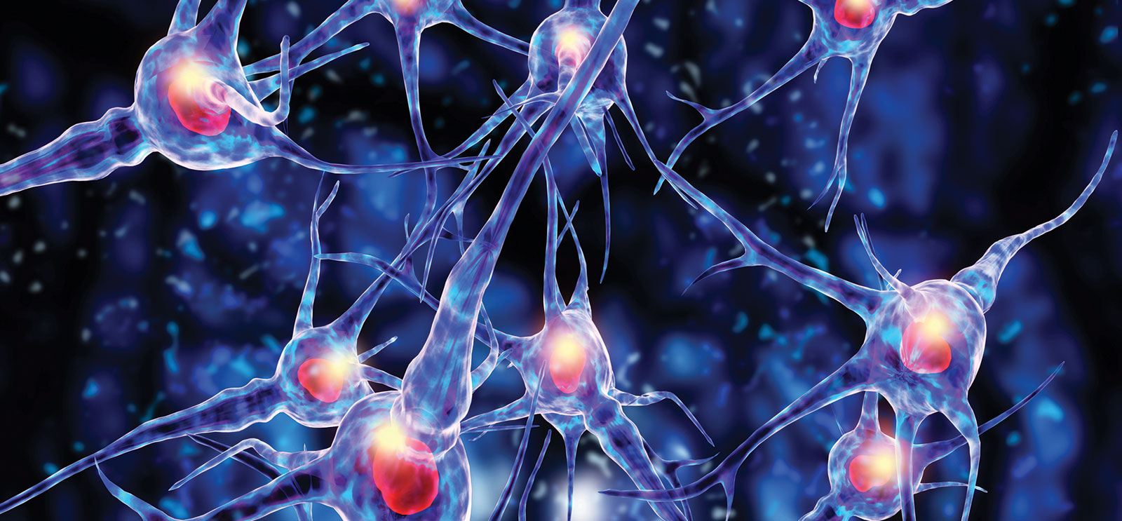
The Human Brain's Neural Network

Each artificial neuron (aka perceptron) in the layers is functionally similar to an actual neuron. An artificial neuron has an input gate and output gate, which corresponds to dendrite and axon terminal respectively. The human brain alters connection strength between each neuron instead of creating a new brain cell to store new information. Artificial neural networks follow this process and update weights, which is one of the core processes of training a deep neural network.

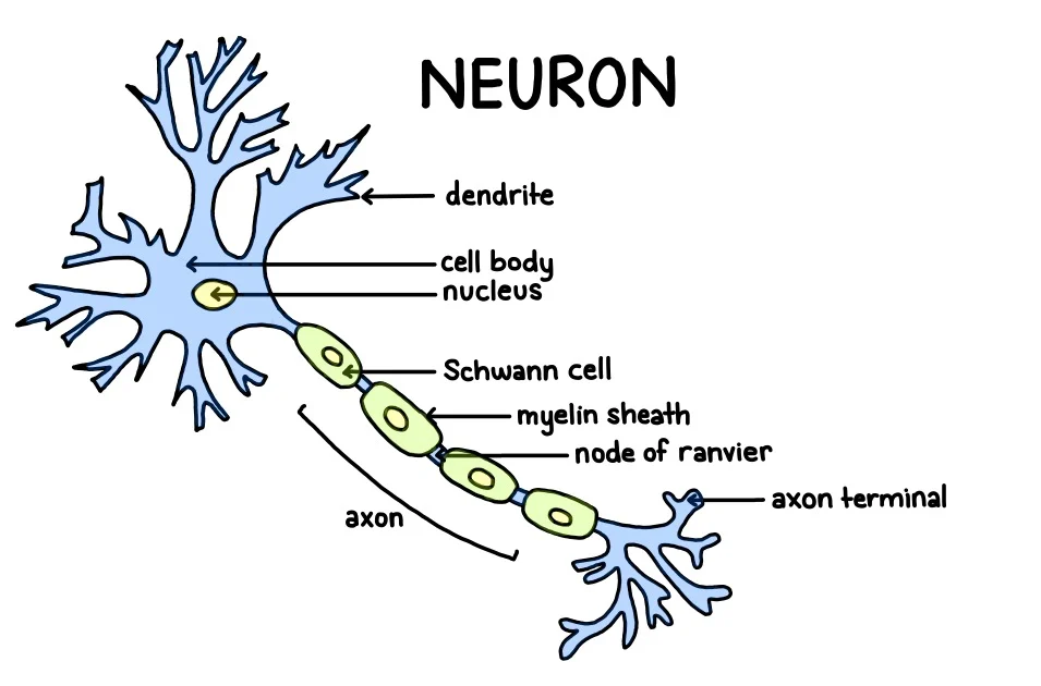
Structure of a Neuron

Perceptrons

Neurons can be represented mathematically as follows.

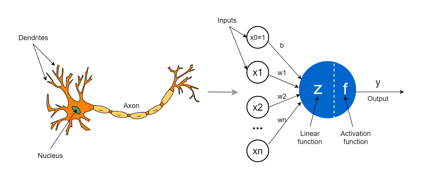
Mathematical Representation of a Neuron

\(x_i\): input (dendrites)
\(w_i\): connection strength/weight (amount of receptors in each dendrite)
\(b\): bias
\(z\) & \(f\): cell body
\(y\): output (axon)

Each input has its own connection weight, and stronger connection strength means more signals can be sent to the next neuron. A neuron here is defined as a cell, not a computer. This means it doesn’t perform heavy calculations or solve complex problems; instead it takes in signals (data) and stores them until it reaches a threshold. We can think of it as a bucket, where signals accumulate until the bucket cannot hold any more, sending them out to the next connected neuron(s). Mathematically, this analogy is expressed as follows.

The first function, equivalent to \(z\) in the above image calculates the weighted sum of inputs. \[ s = x_1w_1 + x_2w_2 + … + x_nw_n = \sum^n_{i=1}x_iw_i \]
The second function, equivalent to \(f\) in the above image evaluates the weighted sum with a non-linear threshold. The example below is a hard limit and in this case the threshold is 0. \[ y = \begin{cases} 1 (s\ge 0) \\ 0 (s<0) \end{cases}\]

Notice that the first function (weighted sum) can also be geometrically interpreted as a linear equation in a 2D space. \[ x_1w_1 + x_2w_2 + w_3 = 0 \] For input values \(x_1\) and \(x_2\), the location of point (\(x_1\), \(x_2\)) would be either above the line, on the line or below the line. If we have a dataset with various inputs, we can interpret them as distinct points on the \(x_1x_2\) plane and line \( x_1w_1 + x_2w_2 + w_3 = 0 \) linearly separating those points.

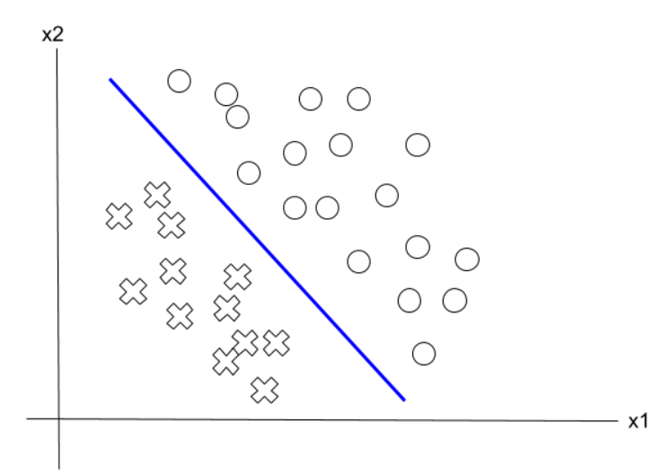
Linearly Separating Samples

Since a perceptron computes the weighted sum of its inputs linearly and applies a threshold to the result, it can only separate data that are linearly separable. As a result, it cannot solve non-linearly separable problems.

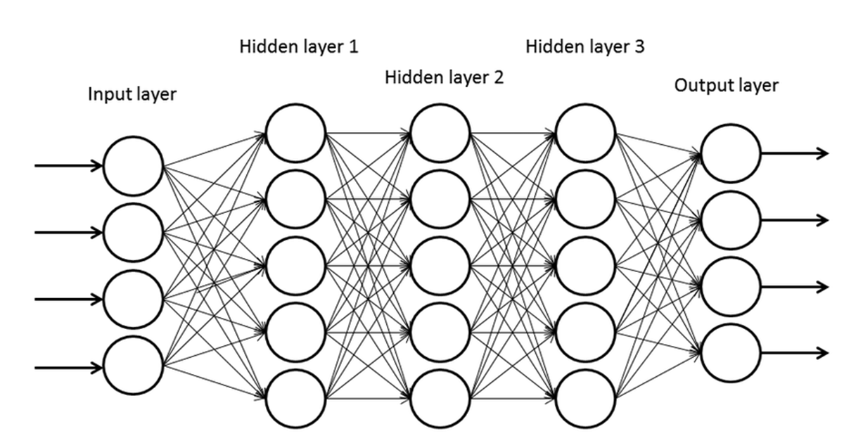
Neural Networks

One common form of a neural network is the multi-layer perceptron (MLP). It stacks multiple layers of perceptrons to solve complex problems. The number of layers and the number of perceptrons in each layer are determined according to the problem and whoever designs the neural network. For complex tasks, adding more layers and a larger number of perceptrons can increase modeling power. However, this may lead to overfitting, which will be addressed in later posts.

Structure of a Multi-Layer Perceptron

One other important factor of a neural network is bias. It is the constant term added at the end of the weighted sum and is included in every layer of a multi-layer perceptron.

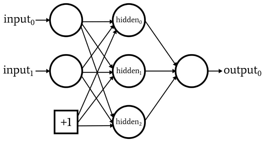
A Network with a Bias Node

Recall that we can geometrically interpret the weighted sum as a linear equation in an \(n\) dimensional space, where \(n\) is the input dimension. In this case, we will assume \(n = 2\) for simplicity.

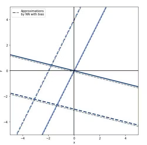
Geometric representation of weighted sum with and without Bias

Without adding a bias, the decision boundary would always have to pass the origin. However, with the bias added to the weighted sum, the boundary can shift freely on the input plane, allowing for a much more flexible model compared to having no bias.