Learning Algorithm
Contents
- Introduction
- Learning with Gradient Descent
- Example of Error Back Propagation
- Generalization & Overfitting
- References
Introduction
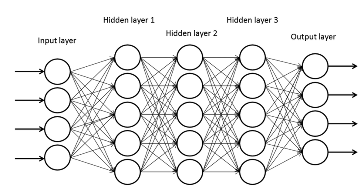
Previously, we discussed how to design a simple neural network. We define a perceptron that computes the weighted sum of inputs and applies a threshold, then sends the resulting value to the next layer. But, we have no idea how to set weights for each connection. This section talks about finding the appropriate weight values with error back propagation.
Learning with Gradient Descent
The basic idea of learning is to find weight values that produce outputs as close as possible to the given (target) outputs. $$ NN(w,x)\approx t\space\space\text{for all}\space (x,t) $$ $$ \Leftrightarrow 0 \approx \sum_{(x,t)\in data}|t-NN(w,x)| $$ $$ \Leftrightarrow 0 \approx \sum_{(x,t)\in data}(t-NN(w,x))^2 $$ $$ \Leftrightarrow E(w) = \sum_{(x,t)\in data}(t-NN(w,x))^2 \space\space\text{minimized} $$
- $x$: input
- $t$: target output
- $NN$: neural network to train
- $E$: loss function
The mathematical problem we need to solve is this.
- Find weights $\textbf{w}=(w_1,w_2, … ,w_n)$ that minimize $E(w) = \sum_{(x,t)\in data}(t-NN(w,x))^2$
To solve this, we take the following steps.
- Randomly initialize $w$
- Find the gradient at the current position
- Move down the loss function along with the gradient
- Repeat until a local minimum is reached.
Gradient Descent
In the steps above, error back propagation is used to compute gradients, and gradient descent is applied to update weights that minimize loss. Note that even though there is some other local minimum or a global minimum that is smaller, the process stops when any local minimum is reached and there is no way to verify whether there is a better minimum. Gradient descent can be mathematically written as follows.
$$ w^{t+1} = w^t - \eta \frac{\partial E}{\partial w}\bigg|_{w=w^t} $$
- $\eta$: learning rate
- $w^t$: current position
- $\frac{\partial E}{\partial w}\bigg|_{w=w^t}$: gradient at current position
The gradient at the current position, multiplied by the learning rate (step size), is subtracted from the current weights, moving the point down the loss function. The learning rate doesn’t need to change for each iteration, because as the weights approach a minimum, the gradient naturally decreases, automatically reducing step size and preventing oscillation. Here is a pseudocode for gradient descent.
Random init w_0, w_1, ...
Repeat
    w_0 = w_0 - lr * dE/dw_0
    w_1 = w_1 - lr * dE/dw_1
    ...
Until stopping condition satisfied
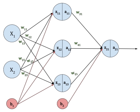
To calculate gradients, we need to differentiate the loss function with respect to each weight. This can be done by getting the partial derivative of the loss function. $$ \frac{dE(w)}{dw_k} = \frac{d}{dw_k} \sum_{(x,t)\in Data}(t-NN(w,x))^2 = \sum_{(x,t)\in Data}\frac{d}{dw_k}(t-NN(w,x))^2 $$
Activation Function
Recall that the cell body of a perceptron computes a linear weighted sum followed by an activation function. According to the chain rule, we need to be able to get a gradient value from every part of the network. Using a hard limit like before would be pointless because it is not differentiable and all gradient values are 0 except for at the threshold. So we replace this with another activation function called the sigmoid function.
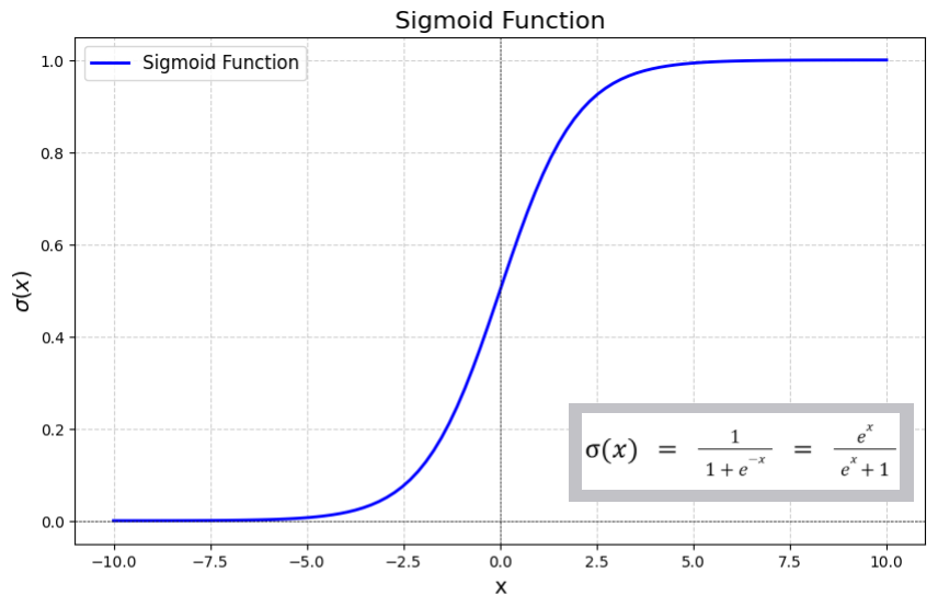
Sigmoid Activation Function
One notable property of the sigmoid function is that its derivative can be expressed in terms of the function itself. $$ \sigma(x) = \frac{1}{1 + e^{-x}} $$ $$ \frac{d}{dx}\sigma(x) = \sigma(x)(1-\sigma(x)) $$ This makes gradient computations convenient in neural networks.
Example of Error Back Propagation
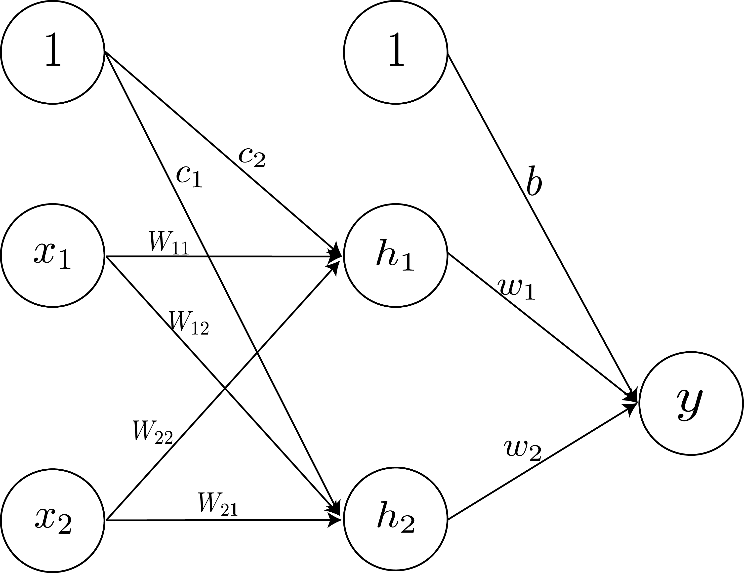
Assume we create a neural network for a XOR logic classifier. Unlike previous simple problems, XOR logic is a non-linearly separable problem, so the network would look something like this.
Sigmoid Activation Function
We’ll then randomly initialize weights like below.
| $x_1$ | $x_2$ | $t$ | $y$ |
|---|---|---|---|
| 1 | 1 | 0 | 0.52 |
| 1 | 0 | 1 | 0.50 |
| 0 | 1 | 1 | 0.52 |
| 0 | 0 | 0 | 0.55 |
Iteration: 0
As we keep updating weights, we can see the expected results getting somewhat close to the target output.
| $x_1$ | $x_2$ | $t$ | $y$ |
|---|---|---|---|
| 1 | 1 | 0 | 0.30 |
| 1 | 0 | 1 | 0.81 |
| 0 | 1 | 1 | 0.81 |
| 0 | 0 | 0 | 0.11 |
Iteration: 3000
| $x_1$ | $x_2$ | $t$ | $y$ |
|---|---|---|---|
| 1 | 1 | 0 | 0.02 |
| 1 | 0 | 1 | 0.98 |
| 0 | 1 | 1 | 0.98 |
| 0 | 0 | 0 | 0.02 |
Iteration: 10000
If we plot the error into a graph, it would look something like this.
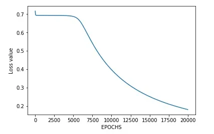
Loss over time
It would be a bad idea to set the stopping condition to when the loss is exactly 0 because
- It would require almost an infinite number of epochs for loss to reach exactly 0.
- Finding weights that have 0 loss for a single sample means it is likely to not perform well with other samples.
Therefore it is crucial to stop training at an appropriate point where the results are appropriate for a general dataset.
Generalization & Overfitting
This brings us to generalization and overfitting. Depending on how we set the hyperparameters, the neural network may perform well on unseen samples or only on those used for training. The former is a neural network with good generalization while the latter is an overfitted neural network. A well-trained neural network not only generalizes the dataset, but also predicts unlearned values well. Our objective is to train a generalized neural network.
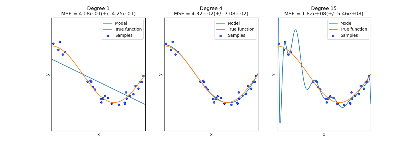
Underfitting, Generalization and Overfitting
The graph on the left is an example of underfitting. The neural network’s modeling power is too weak compared to the complexity of the problem, so a rather simple decision boundary is generated, not being able to predict unlearned samples. The graph on the right is an example of overfitting. It has strong modeling power and is trained extremely well with the given training samples. However, this still doesn’t predict unlearned values well. The graph in the middle is what is generally considered a neural network with the right fit. It generalizes the dataset well and provides highly accurate prediction for new data.
Underfitting usually happens when there aren’t enough layers or perceptrons in the network. This can be fixed by increasing the complexity of the model (number of layers or neurons).
Overfitting happens because it learns the exact training dataset. One might think taking into account all the samples exactly may positively affect the network, but we have to keep in mind that the neural network doesn’t evaluate just the given set; it is trained to predict unknown, new values. By learning the dataset perfectly, it would also mean the neural network has learned the noise that may be present within the data, thus leading to inaccurate prediction of unlearned samples.
To sum up, it is important to find the optimal number of neurons and training iterations. We can also use other techniques like regularization, or get more training data for better generalization.
References
Mathematics behind the Neural Network