Introduction to Machine Learning - Supervised Learning
The contents of this post are lecture notes from professor Andrew Ng’s course, Supervised Machine Learning: Regression and Classification .
Contents
Supervised Learning
Supervised learning is a method of machine learning that learns from data labeled with right answers. Here are some example applications of supervised learning.
| Input | Output | Application |
|---|---|---|
| Spam? (True/False) | Spam Filtering | |
| Audio | Text Transcripts | Speech Recognition |
| Image, Radar info | Position of other cars | Self-driving cars |
There are two types of supervised learning.
Regression is a learning method that predicts a continuous or numeric output value. It is used when the target variable is continuous and has a real number value, like house price prediction and predicting a human’s age based on various features. There are infinitely many possible outputs in regression.
Classification is a learning method that predicts a categorical or discrete output label/class. It is used when the target variable is a category, like spam filtering and image classification. In this case, there are only a small and limited number of possible outputs.
Regression
Linear Regression
As mentioned above, regression learns from right answers. Linear regression is a type of regression that models the relationship between a dependent variable and one or more independent variables with a linear equation. The goal of linear regression is to find the linear equation that best fits the relationship between variables.
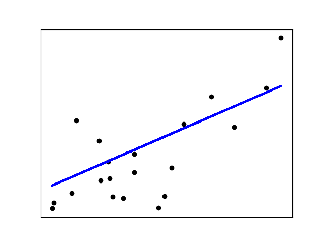
Linear Regression
Linear regression with a single feature \(x\) is mathematically expressed as follows.
$$ f_{w, b}(x) = wx + b $$
- $x$ : input variable feature
- $y$ : output variable feature / target variable
- $\hat y$ : prediction (estimated $y$)
- $m$ : number of training examples
- $(x, y)$ : single training example
- $(x^{(i)}, y^{(i)})$ : $i^{th}$ training example
Cost Function
A Cost Function is a function that quantifies how well a machine learning model’s prediction matches the actual values. The goal is to minimize the cost function, and a cost function with 2 parameters can be visualized with a contour plot. A contour plot with the shape close to a circle has better performance.
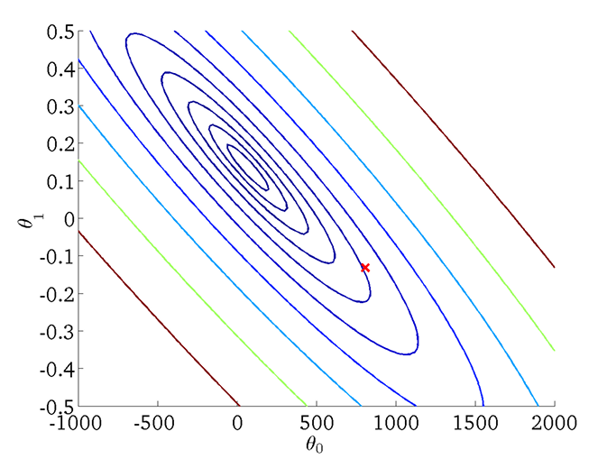
Cost function visualized as a contour plot
The cost function of model $f_{w, b}(x) = wx + b$ is mathematically expressed as follows.
$$ J(w,b)=\frac 1 {2m} \sum_{i=1}^m(f_{w,b}(x^{(i)})-y^{(i)})^2 $$
- $w$ : weight(s)
- $b$ : bias
Gradient Descent
Gradient Descent is an optimization algorithm that minimizes the cost function. The basic idea is to iteratively adjust model parameters and decrease the cost function. The following is a mathematical expression and pseudo code of gradient descent with one weight parameter.
$$ w=w-\alpha \space \frac \partial {\partial w}J(w,b) $$ $$ b=b-\alpha \space \frac \partial {\partial b}J(w,b) $$
Mathematical expression of gradient descent
# Repeat until convergence
tmp_w = w - α * dj_dw
tmp_b = w - α * dj_db
w = tmp_w
b = tmp_b
Pseudo code of gradient descent
$\alpha$ is the learning rate. If the learning rate is too small, the algorithm is slow. If the learning rate is too big, the algorithm may overshoot and fail to converge. Below is the mathematical expression of gradient descent for linear regression.
$$ \frac \partial {\partial w}J(w,b)=\frac 1 m \sum_{i=1}^m(f_{w,b}(x^{(i)})-y^{(i)})x^{(i)} $$ $$ \frac \partial {\partial b}J(w,b)=\frac 1 m \sum_{i=1}^m(f_{w,b}(x^{(i)})-y^{(i)}) $$
Gradient descent of linear regression
Linear Regression with Multiple features
Linear regression can be expressed with multiple parameters. Each parameter represents an individual feature.
$$ f_{\vec{w},b}(\vec{x}) = w_1x_1+w_2x_2+\space … \space+w_nx_n+b $$
- $ \vec{w} = \begin{bmatrix} w_1 & w_2 & w_3 & … & w_n \end{bmatrix}$
- $b$ is a number
- $ \vec{x} = \begin{bmatrix} x_1 & x_2 & x_3 & … & x_n \end{bmatrix}$
Therefore, in vector notation the model can be expressed as
$$ f_{\vec{w}, b}(\vec{x}) = \vec{w} \cdot \vec{x} + b $$
This is also known as multiple linear regression, which is a type of linear regression with two or more independent variables.
Gradient Descent for Multiple Linear Regression
Each iteration of gradient descent for multiple linear regression is expressed as follows.
$$
w_1=w_1-\alpha \space \frac 1 m \sum_{i=1}^m(f_{\vec w,b}(\vec x^{(i)})-y^{(i)})x_1^{(i)}
$$
$$
…
$$
$$
w_n=w_n-\alpha \space \frac 1 m \sum_{i=1}^m(f_{\vec w,b}(\vec x^{(i)})-y^{(i)})x_n^{(i)}
$$
$$b=b-\alpha \space \frac 1 m \sum_{i=1}^m(f_{w,b}(x^{(i)})-y^{(i)})
$$
In each iteration, $w_j\space(j=1\space…\space n)$ and $b$ is simultaneously updated.
- $x_j$ : $j^{th}$ feature
- $n$ : number of features
- $\vec x ^{(i)}$ : features of $i^{th}$ training example (row vector)
- $x_j^{(i)}$ : value of feature $j$ in $i^{th}$ training example
Feature Scaling
Feature scaling is a technique that speeds up gradient descent. Below is a simple example of how it is applied.
$300\le x_1\le 2000, \space 0\le x_2\le5$
$\rightarrow 0.15\le \frac {x_1} {2000}\le 1,\space 0\le \frac {x_2} 5\le1$
$\rightarrow 0.15\le x_1’\le1,\space 0\le x_2’\le1$
Some well known examples of feature scaling are Mean normalization and Z-Score normalization.
$$ 300\le x_1\le 2000, \space 0\le x_2\le5,\space \mu_1 = 600,\space \mu_2 = 2.3 \space \space (\mu_1, \mu_2 \text{ are average of } x_1 \text{ and } x_2) $$
$$ \rightarrow x_1’=\frac {x_1-\mu_1} {2000-300}, \space x_2’=\frac {x_2-\mu_2} {5-0} $$
$$ -0.18\le x_1’\le 0.82, \space -0.46\le x_2’\le0.54 $$
Mean Normalization
$$ x_1 = \frac {x_1-\mu_1} {\sigma_1}, \space x_2 = \frac {x_2-\mu_2} {\sigma_2} \space (\sigma_1, \sigma_2 \text{ are standard deviation of } x_1 \text{ and } x_2) $$
Z-Score Normalization (Standardization)
Feature Engineering
Feature engineering is a process of selecting a set of features and creating new features from them. Below is an example.
$$ f_{\vec w, b}(\vec x)=w_1x_1+w_2x_2+b $$
- $x_1$: frontage
- $x_2$: depth
- $x_3$ : area (frontage * depth) $\rightarrow$ NEW FEATURE
Polynomial Regression
Polynomial regression is a type of regression where the relationship between dependent and independent variable is expressed as an nth degree polynomial.
$$ f_{\vec w, b}(x)=w_1x+w_2x^2+w_3x^3+b $$ $$ f_{\vec w, b}(x)=w_1x+w_2\sqrt x + b $$
Polynomial regression
Classification
Binary Classification
Binary classification is a type of supervised machine learning task where the goal is to categorize data into one of two possible categories/classes/labels. The target variable in this case is binary, meaning it can take only 2 distinct values.
$$ \text{if } f_{w,b}(x)<0.5 \rightarrow \hat y = 0 $$ $$ \text{if } f_{w,b}(x)\ge 0.5 \rightarrow \hat y = 1 $$
Example of binary classification
Logistic Regression
In contrast to linear regression, logistic regression is a type of regression that models the probability of a binary outcome as a function of one or more independent variables or features. The goal of logistic regression is to find the relationship between the independent variables and the probability of a particular outcome. The logistic function, or the sigmoid function is used to model the relationship.
$$ g(z)=\frac 1 {1+e^{-z}} \space(z=\vec w \cdot \vec x + b) $$
Sigmoid function
This can be rewritten as follows
$$ f_{\vec w, b}(\vec x)= g(\vec w\cdot \vec x+b)= \frac {1} {1+e^{-(\vec w\cdot \vec x+b)}} $$
which is equal to the probability that the class is 1.
- $f_{\vec w,b}(\vec x) = 0.7\space$ indicates that there is a 70% chance that \(y\) is 1.
- $f_{\vec w, b}(\vec x) = P(y=1|\vec x;\vec w,b)\space$ indicates the probability that $y$ is 1, given input $\vec x$ and parameters $\vec w$, $b$.
Decision Boundary
A decision Boundary is the boundary or dividing line that separates different classes or categories in a dataset.
$$f_{\vec w, b}(\vec x)=g(z)=g(w_1x_1+w_2x_2+b)$$ $$w_1=1,w_2=1,b=-3$$ $$z=\vec w \cdot \vec x + b = 0$$ $$=x_1+x_2-3 = 0$$ $$\therefore x_1+x_2=3$$
Linear decision boundary
$$f_{\vec w, b}(\vec x)=g(z)=g(w_1x_1^2+w_2x_2^2+b)$$ $$w_1=1,w_2=1,b=-1$$ $$z=x_1^2+x_2^2-1=0$$ $$\therefore x_1^2+x_2^2=1$$
Non-linear decision boundary
Cost Function for Logistic Regression
The loss function for logistic regression $L(f_{\vec w, b}(\vec x^{(i)}), y^{(i)})=$ $$ -log(f_{\vec w, b}(\vec x^{(i)})) \space\space (if\space\space y^{(i)} = 1) $$ $$ -log(1-f_{\vec w, b}(\vec x^{(i)})) \space\space (if\space\space y^{(i)} = 0) $$
-
if $y^{(i)}=1$,
$L(f_{\vec w, b}(\vec x^{(i)}), y^{(i)})= -log(f_{\vec w, b}(\vec x^{(i)}))$
- As $f_{\vec w, b}(\vec x^{(i)}) \rightarrow 1$ then loss $\rightarrow 0$
- As $f_{\vec w, b}(\vec x^{(i)}) \rightarrow 0$ then loss $\rightarrow \infty$
-
if $y^{(i)}=0$
$L(f_{\vec w, b}(\vec x^{(i)}), y^{(i)})= -log(1-f_{\vec w, b}(\vec x^{(i)}))$
- As $f_{\vec w, b}(\vec x^{(i)}) \rightarrow 0$ then loss $\rightarrow 0$
- As $f_{\vec w, b}(\vec x^{(i)}) \rightarrow 1$ then loss $\rightarrow \infty$
This can be simplified as $$L(f_{\vec w, b}(\vec x^{(i)}), y^{(i)})=-y^{(i)}\space log(f_{\vec w, b}(\vec x^{(i)}))-(1-y^{(i)})\space log(1-f_{\vec w, b}(\vec x^{(i)}))\text{ (Convex, Single global minimum)}$$
And therefore the cost function is $$J(\vec w,b)=-\frac 1 m \sum_{i=1}^m[y^{(i)}\space log(f_{\vec w, b}(\vec x^{(i)}))+(1-y^{(i)})\space log(1-f_{\vec w, b}(\vec x^{(i)}))]$$
Simplified cost function for logistic regression
Gradient Descent for Logistic Regression
Gradient descent for logistic regression is performed as follows.
$$w_j=w_j-\alpha \space \frac 1 m \sum_{i=1}^m(f_{\vec w,b}(\vec x^{(i)})-y^{(i)})x_j^{(i)}$$ $$b=b-\alpha \space \frac 1 m \sum_{i=1}^m(f_{w,b}(x^{(i)})-y^{(i)})$$ In each iteration, $w_j\space(j=1\space…\space n)$ and $b$ is simultaneously updated. For logistic regression, $f_{\vec w,b}(\vec x) = \frac 1 {1+e^{-(\vec w \cdot \vec x + b)}}$.
Overfitting and Underfitting
Overfitting is a problem where the machine learning model learns too well and takes into account noise, random fluctuations or anomalies and misses the true pattern. Underfitting is a problem where the model is too simple to capture a pattern in training data. Here is a comparison of each case.

Comparison of underfitting, overfitting and optimal fitting
- Underfit
- High Bias
- Does not fit the training set well
- Overfit
- High Variance
- Fits training set extremely well, but does not work well with new examples that are not in the training set
- Optimal
- Generalizes Well
- Fits training set well
Regularization
Regularization is a technique used to prevent overfitting and improve generalization of a model.
- Cost Function with Regularization
$$J(\vec w, b)=\frac 1 {2m} \sum_{i=1}^m (f_{\vec w,b}(\vec x^{(i)})-y^{(i)})^2+\frac \lambda {2m}\sum_{j=1}^nw_j^2$$
- $\frac \lambda {2m}\sum_{j=1}^nw_j^2$ is the regularization term.
- $\lambda$ is the regularization parameter. $(\lambda > 0)$
- if $\lambda > 0$, it is the same as not using regularization. (overfit)
- if $\lambda = 10^{10}, f(x) \approx b$, model is underfit.
- Regularized Linear Regression
$$w_j=w_j-\alpha \space [\frac 1 m \sum_{i=1}^m(f_{\vec w,b}(\vec x^{(i)})-y^{(i)})x_j^{(i)}+\frac \lambda {m}w_j]$$
$$b=b-\alpha \space \frac 1 m \sum_{i=1}^m(f_{w,b}(x^{(i)})-y^{(i)})$$
One iteration
- $\frac \partial {\partial w_j} J(\vec w,b)=\frac 1 m \sum_{i=1}^m(f_{\vec w,b}(\vec x^{(i)})-y^{(i)})x_j^{(i)}+\frac \lambda {m}w_j$
- $w_j=w_j(1-\alpha \frac \lambda m)-\alpha \space \frac 1 m \sum_{i=1}^m(f_{\vec w,b}(\vec x^{(i)})-y^{(i)})x_j^{(i)}$
- $(1-\alpha \frac \lambda m)$ is a number slightly smaller than 1, so multiplying this to $w_j$ means after every iteration, $w_j$ shrinks slightly.
- Regularized Logistic Regression
$$w_j=w_j-\alpha \space [\frac 1 m \sum_{i=1}^m(f_{\vec w,b}(\vec x^{(i)})-y^{(i)})x_j^{(i)}+\frac \lambda {m}w_j]$$
$$b=b-\alpha \space \frac 1 m \sum_{i=1}^m(f_{w,b}(x^{(i)})-y^{(i)})$$
One iteration
$$J(\vec w,b)=-\frac 1 m \sum_{i=1}^m [y^{(i)}\space log(f_{\vec w, b}(\vec x^{(i)}))+(1-y^{(i)})\space log(1-f_{\vec w, b}(\vec x^{(i)}))]+ \frac \lambda {2m}\sum_{j=1}^nw_j^2$$
Cost function