Deep Learning
Contents
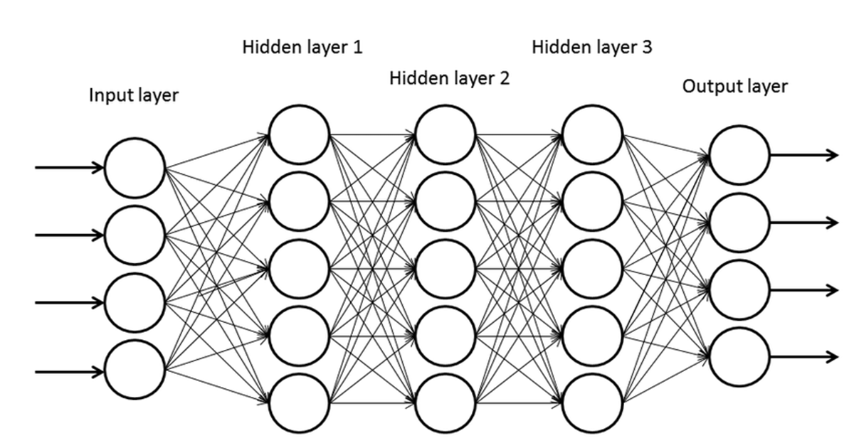
Before 2000, deep neural networks could not be trained because computational costs were extremely high and none of the hardware back then could handle such intensive computation. By 2010, deep neural networks—a neural network with a lot of hidden layers—could be trained effectively. Compared to shallow networks, deep neural networks are more expressive and are capable of solving complex problems. However, naively increasing the number of layers and making the neural network deeper will cause problems in training. Deeper networks are prone to overfitting, and also have the vanishing gradient problem. In this post, we will discuss vanishing gradients and its solution, along with dropout which mitigates overfitting and finally batch normalization which solves the internal covariate shift problem.
Vanishing & Exploding Gradients
Previously, we frequently used the sigmoid activation function for our non-linear transformation in neural networks. One property of the sigmoid function is that its range is always (0,1). If the network gets deeper, it means activations are repeatedly multiplied through the chain rule and here is where the issue arises. Multiplying a value in the range (0,1) several times will cause the value to converge to 0. But the gradient has a multiplicative sigmoid derivative at each activation, since the derivative of sigmoid is
$$ \frac{\partial}{\partial x}\sigma (x) = \sigma (x) (1-\sigma (x)) $$
The gradient will then converge to 0 and the network will be unable to learn, since the gradient is near 0.
Similarly, if the gradient values are extremely big for various layers, the value may exponentially increase and become infinity or NaN, thus unable to train. This is called the exploding gradient problem.
Rectified Linear Unit (ReLU)
Since the derivatives of the activation function are the major terms of gradients, we can prevent gradient vanishing by replacing the sigmoid activation with another non-linear function. This is where we use ReLU (Rectified Linear Unit). ReLU is defined as follows.
$$ f(x) = \begin{cases} x\space (x > 0) \\\\ 0\space (x\le 0) \end{cases} $$
Its derivative will then become
$$ \frac{d}{dx}f(x) = \begin{cases} 1\space (x > 0) \\\\ 0\space (x\le 0) \end{cases} $$
Now every term which was the derivative of sigmoid is now replaced with 1 or 0. The values are binary, which is now simpler and lightweight, preserving previous gradient values. It is also non-linear, so it satisfies the non-linearity condition needed in activation functions.
ReLU significantly reduces the vanishing gradient problem and is computationally much more efficient than the sigmoid activation function. Despite these advantages, ReLU still has problems in very deep neural networks because they still suffer from optimization issues when the network has too many layers. This problem will be discussed in a future post.
The dying ReLU problem (aka knockout) is also an issue with ReLU because if all data have negative values, every gradient will be 0, thus making it impossible to learn. Alternative activation functions like Leaky ReLU and Swish are introduced for this reason.
Even with these issues, ReLU has become a de facto standard for activation functions and is now almost always used for the activation function of hidden layers.
Regularization
Another common problem when training neural networks is overfitting. Overfitting happens because either the neural network is trained too much, or the structure of the neural network is too complex. The former issue can be solved with early stopping, while the latter can be dealt with several approaches like weight decay, dropout, drop connect and stochastic pooling.
Early Stopping
Early stopping is literally stopping early, before the neural network gets overfitted. We know that training too much causes overfitting because it perfectly learns the given dataset, including any noise within the dataset. But how do we know at which point the model starts overfitting? At some point in training, the neural network model will give inaccurate results, meaning its error will increase at some point. But this is only the case when new data is given as input.
To determine when to stop and evaluate the neural network’s error properly, we need to use a portion of the dataset for training and another portion of data to set the stop point and another portion to evaluate those results without biased estimation. Each are called the training set, validation set and test set. The dataset can be split into 6:2:2, 7:1.5:1.5 or 8:1:1.
The training dataset is used for the actual training process. Each epoch consists of multiple gradient descent updates over mini-batches. At the end of an epoch, the validation set is used to determine the stop point. When the stop point is determined and training is terminated, the test set is used to evaluate the results.

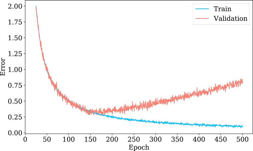
Training Error and Validation Error
In the image above, we can observe that the validation error increases at approximately 150 epochs, which indicates that the model has started to overfit. We can conclude that small training error does not always imply good performance and an evaluation is needed to ensure accuracy.
Weight Decay
Weight decay is another regularization method that adds penalties for large weights to the loss function. L1 regularization and L2 regularization are types of weight decay and each method affects weights differently.
L1 regularization penalizes the absolute value of weights and pushes many weights to zero. Some features may be completely ignored during the process. Optimization is less smooth in L1 regularization and can be unstable when features are highly correlated.
$$ \tilde E(w) = E(w) + \lambda\sum|w_i| $$
L1 Regularization
Reducing the sum of absolute values of weights increases zero connections and therefore leads to a simpler neural network.
L2 regularization penalizes peaky weights and focuses on the square of weights. Like L1 regularization, it also pushes weights to 0, but does not make it exactly 0. Compared to L1 regularization, optimization is smoother and generally produces better results.
$$ \tilde E(w) = E(w) + \frac{\lambda}{2}\sum w_i^2 $$
L2 Regularization
In both equatons, $\lambda$ is the regularization strength. The larger the value, the stronger the regularization and higher risk of underfitting.
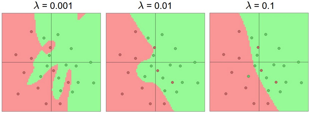
L2 Regularization Strengths of 0.001, 0.01 and 0.1
L2 regularization encourages using all input features by shrinking weights smoothly rather than driving them to zero, unlike L1 regularization which promotes sparsity. Both L1 and L2 introduce a model complexity tradeoff, but L2 is generally preferred for training large deep neural networks due to its smoother optimization and better numerical stability.
We can use $\sum |w_i|$ or $\sum w_i^2$ to measure model complexity. Large weight norms indicate stronger model capacity and sensitivity, while small norms indicate smoother, more regularized models.
Dropout
Another method to reduce structural complexity without removing nodes is dropout. Dropout achieves structural complexity reduction without removing nodes by randomly dropping nodes with a probability.
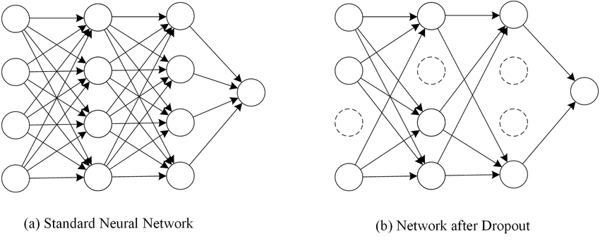
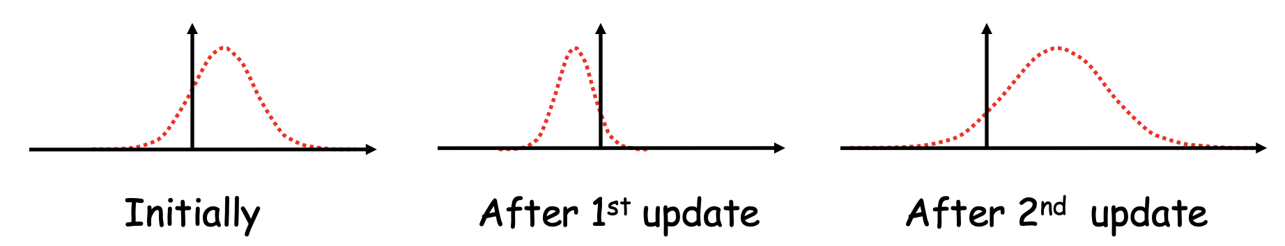
Dropout Neural Network Model
In each update, we drop certain nodes with the predefined probability, disabling them temporarily. Weights connected to active neurons are updated in each iteration of the training loop. In the testing phase, all nodes are used without dropout since the final model utilizes all nodes.
Generally, applying dropout slows training by roughly 2-3x compared to training without dropout, but it excels when the data is not big enough. When very large datasets are available, the regularization benefit of dropout is often reduced.
Batch Normalization
During training, the distribution of a node’s output changes as the parameters of previous layers are updated. These shifts accumulate over iterations, and consequently this has a similar effect to using different training samples at every iteration, which slows and destabilizes training.
Internal Covariate Shift
Therefore, it is reasonable to normalize pre-activation values. We add a normalization layer to each network layer and apply it in between the linear sum and activation. In the normalization layer, each linear sum is z-transformed and a learnable scale and shift parameter is added.
$$ net = \textbf{W}\textbf{x} $$
Summation
$$ \hat {net} = \frac{net-\mu}{\sqrt{\sigma^2+\epsilon}} $$ $$ \tilde {net} = \gamma \hat {net} + \beta $$ $$ \beta, \gamma \space\text{are trainable parameters} $$
Normalization
$$ f(\tilde{net}) $$
Activation
One thing to note is that during z-transformation, subtracting the batch mean cancels out the bias term, so we add a learnable parameter $\beta$ to function just like the bias. Also, batch normalization requires storing statistics of each mini batch during training, resulting in an additional memory overhead.
As mentioned, the mean and variance of each batch are used for normalization, but testing cannot take the same approach since it is using a single sample at a time. Instead, we use the running mean and running variance accumulated during training for normalization at test time.
$$ \hat x = \frac{x-\mu_{running}}{\sqrt{\sigma_{running}^2+\epsilon}} $$
Mean and Variance for Testing
Batch normalization mitigates the internal covariate shift problem and reduces the dependence of gradients on the scale of connection weights.
References
Overview of Machine Learning Part 1 Figure 4
Lecture Slides of Introduction to Deep Neural Networks, lectured by Professor Jee-Hyong Lee
Lecture 27: Linear Classifiers 3/Neural Nets 1
Multiple Instance Fuzzy Inference Neural Networks - Fig 4