Configuration of Neural Networks
Contents
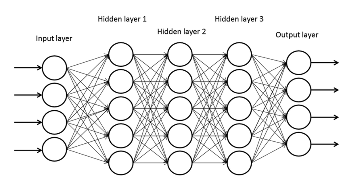
In previous posts, we discussed the basics of neural networks and how to train one. In this post, we will talk about the 3 different types of prediction problems a neural network can handle and how to configure a neural network to solve them.
Regression
Regression refers to predicting a real value for a given input. For example, given engine size, horsepower, vehicle weight and year of car, a regression problem predicts fuel efficiency (miles per gallon).
$$
\begin{bmatrix}
2.0 & 150 & 3000 & 2015 \\\
2.4 & 180 & 3200 & 2016 \\\
1.8 & 130 & 2800 & 2013 \\\
3.0 & 200 & 3500 & 2017 \\\
2.5 & 170 & 3300 & 2014 \\\
1.6 & 110 & 2600 & 2012
\end{bmatrix}
\Rightarrow
\begin{bmatrix}
25.5 \\\
24.0 \\\
28.7 \\\
22.2 \\\
23.8 \\\
30.1
\end{bmatrix}
$$
But recall that we had an activation function for every neuron and we used a sigmoid function for each of them. The sigmoid function returns a real number between 0 and 1, which may not be as useful in many cases.
The solution is to change the activation function of the output node into a linear function. This removes the restriction of the output being between 0 and 1. But since the weighted sum is also a linear representation of values from previous layers, it would be perfectly fine to just remove the output node’s activation function.
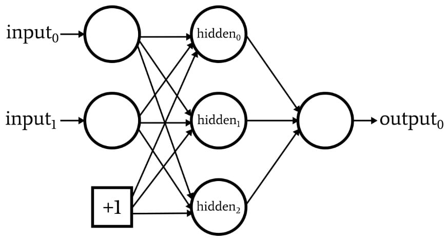
Let $y$ be the output value of the neural network, and $y_1$, $y_2$ be the output values of the hidden layer. Assuming bias exists, the weighted sum of the output node would be $$ y = y_1w_1 + y_2w_2 + w_3 $$
The range of $y_1$ and $y_2$ is between 0 and 1 because it is the result of a sigmoid function and $w_1$, $w_2$ are both real numbers. Therefore, the weighted sum of the output node is a real number and the neural network will work fine without an activation function in the output node. We can also say that removing the activation function has the same effect as using a linear activation function.
We can also express the process with matrices.
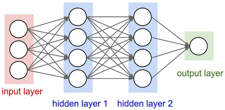
Let the input layer have inputs $x_i$, hidden layer 1 have weighted sum $s_i$, return value $h_i$ and hidden layer 2 have weighted sum $\sigma_i$, return value $H_i$ and $y$ be the output value, where $i$ is the index of each node in a layer. We can express them as vectors, and with each step, the vector is being transformed into another vector. $$ \begin{bmatrix} x_1 \\\\ x_2 \\\\ x_3 \end{bmatrix} \Rightarrow \begin{bmatrix} s_1 \\\\ s_2 \\\\ s_3 \\\\ s_4 \end{bmatrix} \rightarrow \begin{bmatrix} h_1 \\\\ h_2 \\\\ h_3 \\\\ h_4 \end{bmatrix} \Rightarrow \begin{bmatrix} \sigma_1 \\\\ \sigma_2 \\\\ \sigma_3 \\\\ \sigma_4 \end{bmatrix} \rightarrow \begin{bmatrix} H_1 \\\\ H_2 \\\\ H_3 \\\\ H_4 \end{bmatrix} \Rightarrow … \Rightarrow y $$
Each step is a linear or non-linear vector transformation. The two-lined arrow indicates a linear transformation and the single-lined arrow indicates a non-linear transformation. A simple weighted sum can be expressed as a linear transformation like below.
$$
\begin{bmatrix}
w_{11} & w_{12} & w_{13} & w_{14} \\\
w_{21} & w_{22} & w_{23} & w_{24} \\\
w_{31} & w_{32} & w_{33} & w_{34}
\end{bmatrix}^T
\begin{bmatrix} x_1 \\\\ x_2 \\\\ x_3 \end{bmatrix} =
\begin{bmatrix} s_1 \\\\ s_2 \\\\ s_3 \\\\ s_4 \end{bmatrix}
$$
Transforms by activation are non-linear transformations and therefore cannot be expressed in terms of matrices. To sum up, a neural network consists of linear transformations and non-linear transformations. Linear transforms can be removed, as in the case of the output nodes mentioned above, but non-linear transformations cannot be omitted.
What if a neural network only has linear transformations? With only linear transforms, a neural network is equivalent to a single perceptron and can only solve linearly separable problems. Since all transformations are linear, we can express each transformation as a matrix.
$$ \textbf{x} \cdot \textbf{M}_1 \cdot \textbf{M}_2 \cdot … = y $$
Let $\textbf{x}$ be the input vector and $\textbf{M}_i$ be the matrices for each transformation. All transforms can be expressed as a single matrix $\textbf{M}$, which is equivalent to a single transformation.
$$ \textbf{M} = \textbf{M}_1 \cdot \textbf{M}_2 \cdot … $$
$$ \textbf{x} \cdot \textbf{M} = y $$
Therefore, we should only use non-linear functions for activation functions and the non-linear transformations are much more important in a neural network. Non-linear functions include sigmoid functions, $x^2$, $x^3$ etc.
Binary-Class Classification
A binary class classification problem chooses one of two categories for a given input. An example would be predicting whether a student passes or fails a course depending on score, attendance, homework and participation.
$$
\begin{bmatrix}
85 & 90 & 8 & 80 \\\
60 & 75 & 5 & 60 \\\
78 & 85 & 7 & 70 \\\
45 & 60 & 3 & 50 \\\
90 & 95 & 9 & 85 \\\
50 & 65 & 4 & 55
\end{bmatrix}
\Rightarrow
\begin{bmatrix}
Pass \\\
Fail \\\
Pass \\\
Fail \\\
Pass \\\
Fail
\end{bmatrix}
$$
However, since a neural network cannot output categorical values, we must preprocess the labels into numbers. In this case we will change pass and fail to 1 and 0 respectively. The sigmoid function in the output node gives a value between 0 and 1, e.g. 0.7. Since it’s note exactly 0 or 1, we cannot directly assign it to a class. The solution is to interpret the output value as a probability. If the neural network outputs 0.7, we can say this student has a 70% chance of passing this course.
Since we are interpreting the output differently, we also need to make changes in the training process. In prior examples, we used mean squared error to calculate the loss and gradient. We chose mean squared error because it allows us to directly find weights that minimize the difference between the returned value. However, in this case since we are aiming to maximize the probability that the neural network correctly predicts the training data, we must find weights that maximize the following.
$$ (\prod_{(x,1)\in Data}NN(x;w)) \times (\prod_{(x,0)\in Data}(1-NN(x;w))) $$
This is equivalent to finding weights that minimize $$ E = -\sum^N_{n=1}(t_nlog(y_n) + (1-t_n)log(1-y_n)) $$ We call this cross entropy loss and there is good post about deriving back propagation with cross entropy here, written by Essam Wisam. Differentiation of cross entropy loss looks like this. $$ … $$ $$ E = -(y_tlog(y) + (1-y_t)log(1-y)) $$ $$ \frac{\partial E}{\partial w_2} = \frac{\partial E}{\partial y} \frac{\partial y}{\partial s_2} \frac{\partial s_2}{\partial w_2} = -(\frac{y_t}{y}-\frac{1-y_t}{1-y})y(1-y)h $$ $$ = (-y_t(1-y) + (1-y_t)y)h $$
One reason why we don’t use mean squared error is because during training, mislearned data can cause the neural network get stuck. Assume an extreme case where the target output is 1 but the neural network gives 0 instead. $$ s_1 = x_t \cdot w_1 $$ $$ h = sigmoid(s_1) $$ $$ s_2 = h \cdot w_2 $$ $$ y = sigmoid(s_2) $$ $$ E = \frac{1}{2}(y_t-y)^2 $$ $$ \frac{\partial E}{\partial w_2} = \frac{\partial E}{\partial y} \frac{\partial y}{\partial s_2} \frac{\partial s_2}{\partial w_2} = -(y_t - y)y(1 - y)h $$
- $x_t$: input
- $y_t$: target output
If $y=0$, the gradient is 0. This will stop the training. In normal cases, this would mean the training is done, but in this case it will learn wrong information. Therfore, we use cross entropy loss instead of mean squared error in binary class classification.
In summary, to configure a neural network to solve a binary-class classification problem, we need to preprocess the data into real numbers, apply a sigmoid function at the output node and use cross entropy loss for training.
Multi-Class Classification
What if we have more than two classes to choose from? Suppose we need to determine whether a picture shows a cat, a dog, or a bird based on its size, weight, and age.
$$
\begin{bmatrix}
30 & 5 & 2 \\\
50 & 20 & 3 \\\
15 & 0.2 & 1 \\\
35 & 7 & 4 \\\
60 & 25 & 6 \\\
10 & 0.1 & 0.5
\end{bmatrix}
\Rightarrow
\begin{bmatrix}
Cat \\\
Dog \\\
Bird \\\
Cat \\\
Dog \\\
Bird
\end{bmatrix}
$$
Just like we did in binary class classification, we need to preprocess our data into a format the neural network can use. If we take the same approach, we can handle the nominal values with linear conversion. We can convert cat, dog and bird to 0, 0.5 and 1 respectively, then apply the sigmoid function as the activation function to the output node. It seems reasonable, but there is a problem with this method. Cat, dog and bird do not have a hierarchical order. They are different labels within the same ‘species’ class. labeling them as 0, 0.5 and 1 sets a hierarchy, and this changes the original problem. Instead of linear conversion, we can preprocess the data using one-hot encoding. Since we have 3 categories, we can convert each class into a 3 dimensional vector like below.
- Cat: $[ 1 \space\space 0 \space\space 0 ]$
- Dog: $[ 0 \space\space 1 \space\space 0 ]$
- Bird: $[ 0 \space\space 0 \space\space 1 ]$
We can see that each class now has the same distance and to match this format, we can change the number of outputs to the dimension of the classes. This is also equivalent to performing binary classification on each dimension.
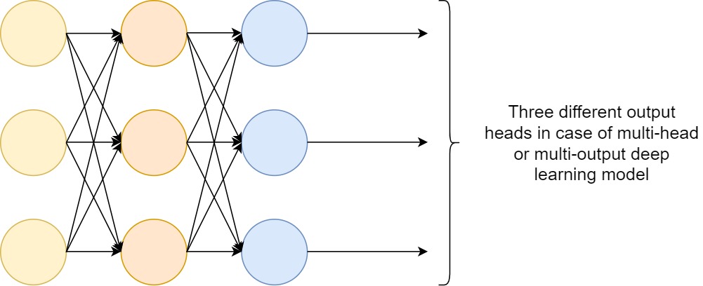
Now since we have three different outputs, an intuitive way of choosing the final class would be to choose the node with the largest value. This means the node with the largest value has the highest probability of being that class. However, a max function is not differentiable and not appropriate for training. We will instead use a function called the softmax function. $$ (y_1,y_2,y_3) = softmax(x_1,x_2,x_3) $$ $$ y_k = \frac{e^{x_k}}{\sum^n_{i=1}e^{x_i}} $$ The softmax function is a non-linear, differentiable activation function and it takes exponentials of the output values because it yields results closer to the original max function. Note that the sigmoid activation function in the output nodes is a monotonically increasing function, so applying it to a max function would be equivalent to not applying the sigmoid activation function.
One reason why we don’t use the sigmoid function as the final activation is because the outputs are probabilities, and their sum must equal 1. The sigmoid function just outputs any value between 0 and 1, while the softmax function always sums up to 1.
Cross entropy loss for multi class classification is as follows. $$ E = \sum^{Data}_{n=1}\sum^{Class}_{k=1}-t_{nk}log(y_{nk}) $$
Summary
We’ve discussed regression, binary class classification and multi class classification in this post. Here is a summary of the activation functions and loss functions for each problem.
| Problem | Hidden Layer | Output Layer | Loss Function |
|---|---|---|---|
| Regression | ReLU | Linear | MSE |
| Binary Class Classification | ReLU | Sigmoid | CE |
| Multi Class Classification | ReLU | Softmax | CE |
References
Getting started with Neural Network for regression and Tensorflow
Multi-Head Deep Learning Models for Multi-Label Classification