Convolutional Neural Networks
Contents
Introduction
We’ve done classification on numerical data, like a simple animal classifier with properties like size, weight and age. But how can we classify a dataset that consists of images? The same approach has limitations, since images are a group of pixel values on a grid, which makes it different from simple numeric properties. We need a different method that takes the structure and characteristics of an image into account.
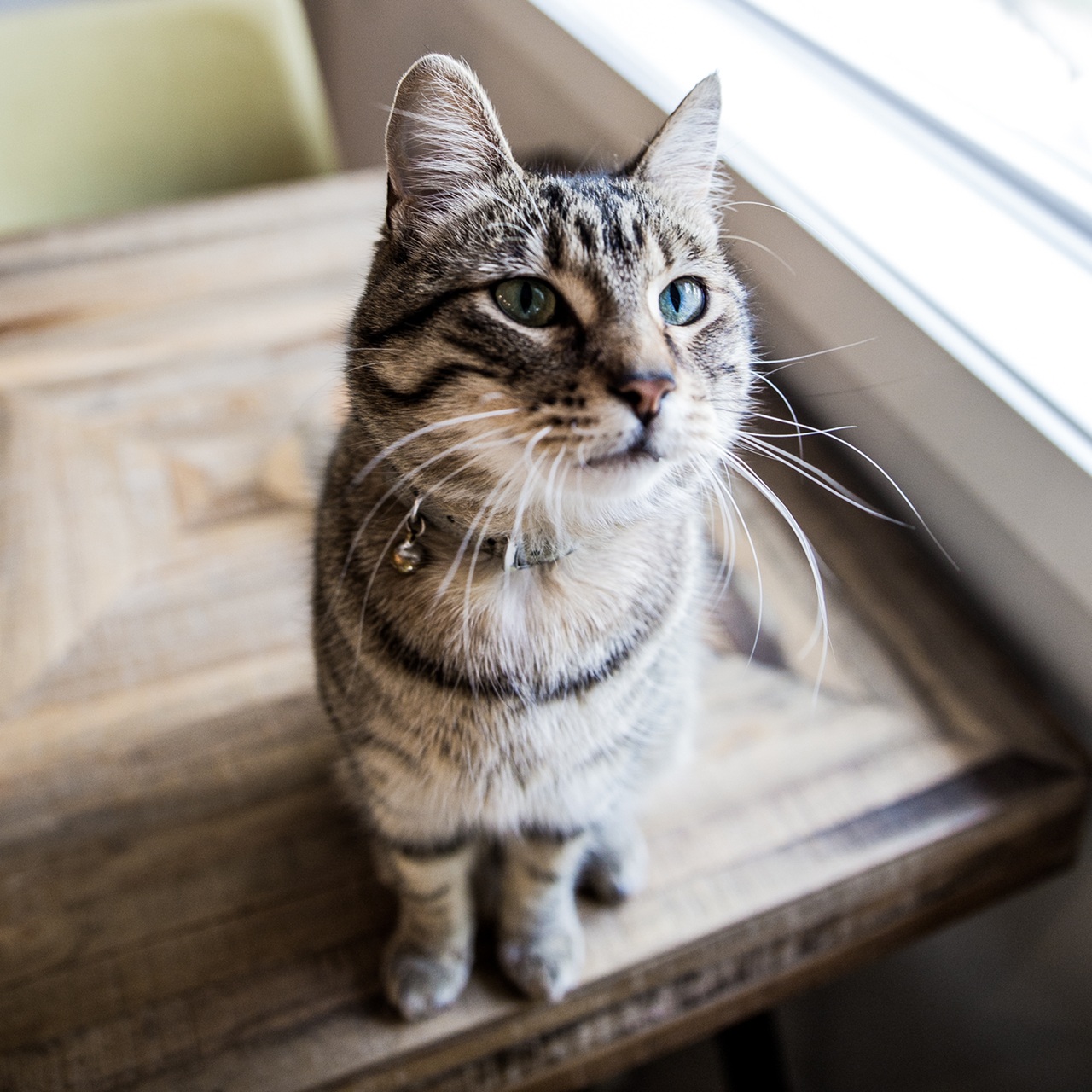

Images of Cats
Think about how humans recognize an image. How do we know these are images of cats? In a split second, we see the eyes, ears, nose, mouth, whiskers, fur, paws and the body of the cat. We put them all together and say it’s a cat.
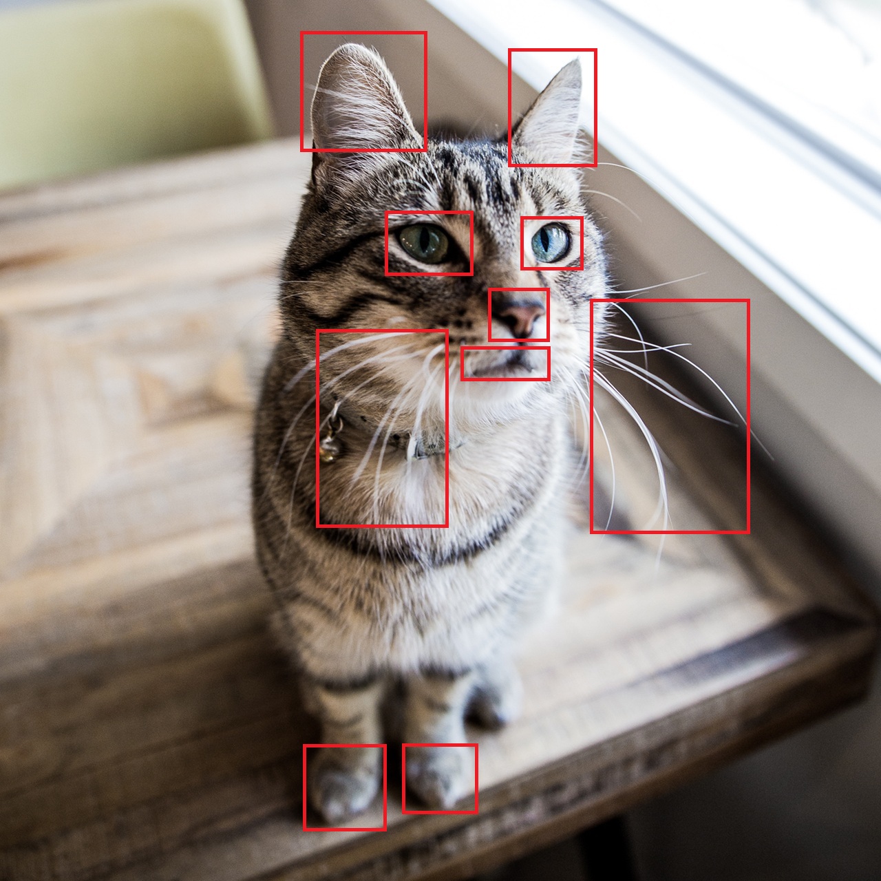
Finding Local Features of Cats
The same approach can be taken with neural networks. We refer to these detected characteristics as local features. Images of the same class tend to share critical local features, which can be used to classify images. A convolutional neural network is designed for this type of problem; it learns spatially local or hierarchical features from grid structured data like images.
Structure of a Convolutional Neural Network
Feature Extraction
Local features can be extracted with a method called convolution. This is done in analogy to computing the dot product to get vector similarity. Intuitively, this can be viewed as a form of local similarity, computed by element-wise multiplication of two matrices followed by a summation.
$$ I * K = \sum K_{ij} \times I_{ij} $$
Convolution
This element-wise multiplication followed by a summation is performed at each spatial location in the image, with the center of the kernel aligned to the corresponding pixel of the input image. The result of each kernel position is then written to the corresponding pixel location in the output feature map.
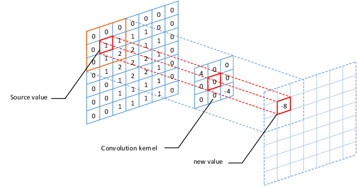
Convolution
For pixels near the image border, zero padding is applied so the kernel can be centered at those locations and the same operation can be done.
Notice that the outcome of the convolution is called a feature map. We extracted local features and encoded them into an output image. Each pixel contains information about the local feature as well as its spatial location. Since this tells us which feature(s) are present and where they are located, it is called a feature map.
Most images have 3 color channels, meaning there are 3 separate grids defined in a single image. Convolution can be applied to each channel by using a filter with the same number of channels.
Pooling
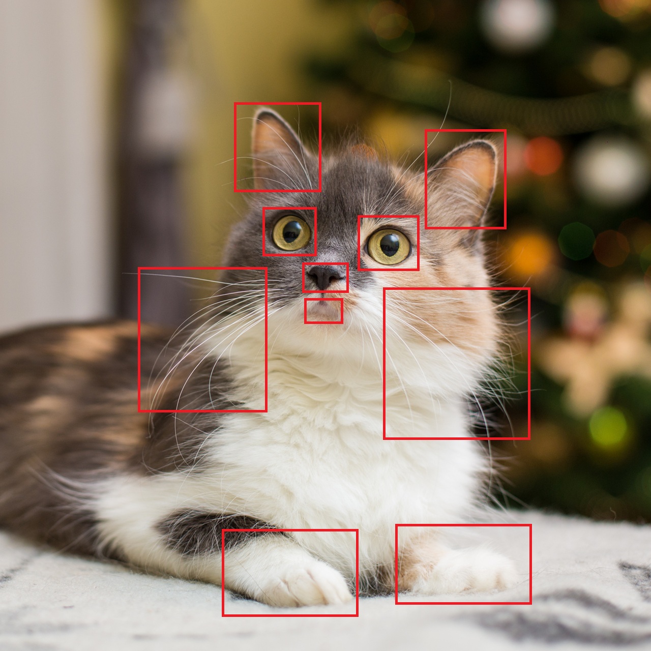
After applying a convolution, we can use a subsampling technique like pooling to reduce the spatial dimension of output features. This process may seem unnecessary, but it has several important advantages.
Pooling provides robustness to small spatial changes. In actual datasets, objects are rarely in the same location, as you can see by the cat images in the beginning of this post. We still recognize them as cats, even though each feature is located differently. If pooling isn’t applied, every feature will be tied to a very specific location, making features dependent on their spatial position. Pooling groups nearby activations into regions, thus giving a more general indication of where a feature lies in the input image.
One other advantage of pooling is reducing computational cost. Since we use several layers of convolution in a convolutional neural network, convolution is applied across multiple layers. If we propagate full-size feature maps continuously, the training process may become computationally heavy. Although subsampling inevitably causes information loss, it is reasonable to reduce the spatial size (height, width) to a range where it does not lose too much feature information.
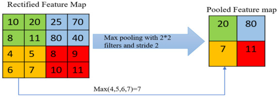
Max Pooling
Max pooling is one of the most commonly used pooling techniques, where the maximum value of a group of pixels corresponding to the kernel is picked and the rest is discarded.
Using the procedure explained above, a filter (or kernel) performs convolution followed by an activation function. Subsampling is optionally done afterwards to reduce the spatial resolution of the feature maps. As mentioned above, the number of input image channels determines the number of channels a filter has, and the number of filters determines the number of output feature map channels. Therefore, the number of trainable parameters for a single convolution layer can be calculated as follows.
$$ N_p = N_{ic} \times K_w \times K_h \times N_o $$
Number of Trainable Parameters in a Single Convolution Layer
where $N_p$ is the number of trainable parameters, $N_{ic}$ is the number of input feature channels, $K_w$ is the kernel width, $K_h$ is the kernel height and $N_o$ is the number of output features. Bias terms are omitted for simplicity.
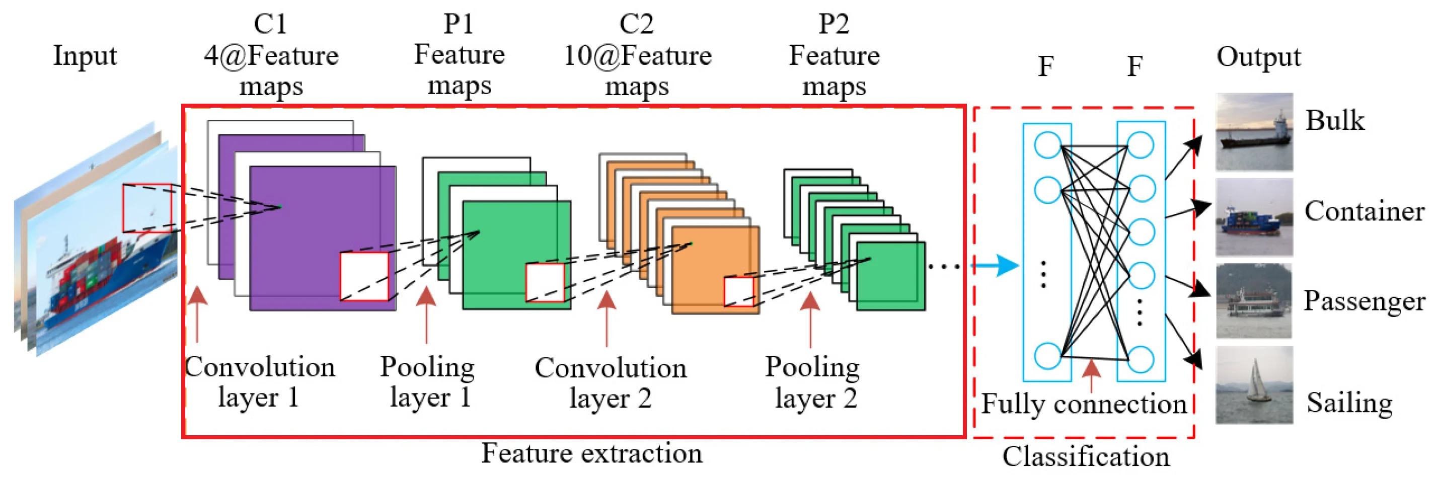
Feature Extraction Phase
A feature map produced by a single filter indicates nearby spatial locations where a feature may be present in the input image. Multiple layers like these are stacked and form the feature extraction phase of a convolutional neural network. In practice, 32 ~ 512 filters are used in a single convolution layer and each perform a convolution.
Classification
At the end of the feature extraction phase, a fully connected neural network is added to perform classification with the extracted features. Each feature map is flattened into a vector and is passed to a fully connected layer. For this reason, pooling is crucial because reducing the spatial dimension reduces the dimension of the input vector of a fully connected layer, thus reducing the number of trainable parameters. The number of trainable parameters in the classification head will be discussed further in the next post.
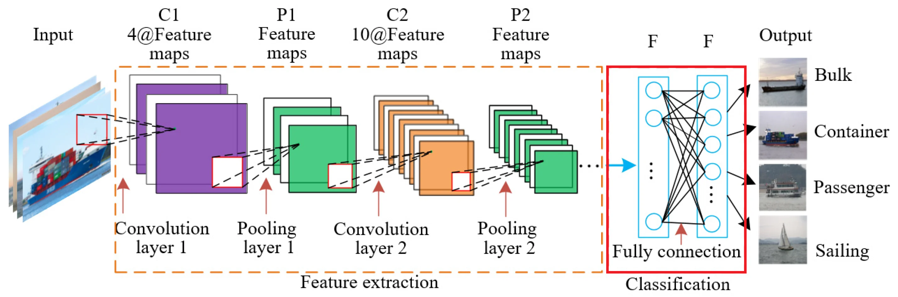
Classification Head
Some additional notes on the structure of the feature extraction phase of a convolutional neural network:
- A single convolution layer corresponds to a single neural network layer.
- For each input feature map of a convolution layer, zero padding can be applied so that kernels can be centered at border pixels.
- Each hidden layer extracts higher level local features from the feature maps produced by the previous layer.
- Each layer outputs a set of feature maps composed of local features.
- The number of pooling operations must be adjusted with respect to the model architecture. Too much pooling will cause greater loss of information.
- Each filter is learned through training.
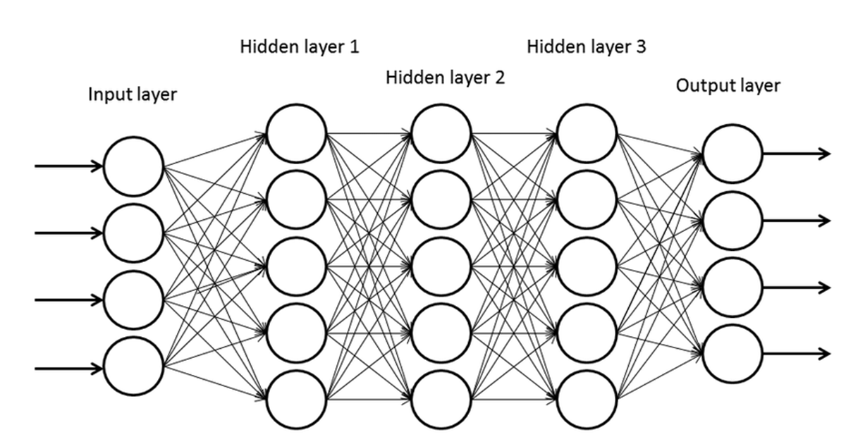
Neural Network Representation
A convolutional neural network can be viewed as a neural network with constrained connectivity and shared weights. Each output pixel corresponds to a pixel in the output feature map and the kernel values correspond to shared connection weights. We can think of it as shared weights in a fully connected neural network because the same set of kernel values are used for every pixel, which corresponds to each input node. Input image pixels that are not multiplied in a convolution can be regarded as disconnected, or a node connected with a weight of 0. Therefore we may conclude that a convolutional neural network can also be represented as a partially connected neural network.
References
Images from Freepik, (bantersnaps, diana.grytsku)